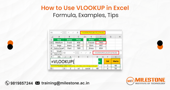
How to Use VLOOKUP in Excel: Formula, Examples, Tips
VLOOKUP is one of the most powerful functions in Excel, enabling users to look up data from a specific column in a table and return a value from another column in the same row. Whether you're managing a budget, tracking sales, or analyzing data, mastering VLOOKUP can significantly enhance your productivity. In this blog, we will explore the VLOOKUP function, how to use VLOOKUP function in excel, its syntax, practical examples, and some useful tips to get the most out of this essential tool.
Understanding VLOOKUP
VLOOKUP stands for "Vertical Lookup." It searches for a value in the first column of a range and returns a value in the same row from a specified column. The function is particularly useful when working with large datasets where finding specific data points manually would be time-consuming.
Syntax of VLOOKUP
The basic syntax of the VLOOKUP function is as follows:
VLOOKUP(lookup_value, table_array, col_index_num, [range_lookup])
lookup_value: The value you want to search for in the first column of the table.
table_array: The range of cells that contains the data. This can be a named range or a reference to a range.
col_index_num: The column number in the table_array from which to retrieve the value. The first column is 1, the second is 2, and so on.
[range_lookup]: This is optional. Use FALSE for an exact match or TRUE for an approximate match (default is TRUE).
Example of Using VLOOKUP
Let’s consider a practical example to illustrate how VLOOKUP works. Imagine you have a table containing product details with their IDs, names, and prices:
Finding Product Price
Suppose you want to find the price of the product with ID 1002 (Smartphone). The VLOOKUP formula would look like this:
=VLOOKUP(1002, A2:C4, 3, FALSE)
lookup_value: 1002 (the Product ID we’re searching for).
table_array: A2
(the range of the product table).col_index_num: 3 (since we want to return the price, which is in the third column).
[range_lookup]: FALSE (we want an exact match).
When you enter this formula, Excel returns ₹45000 ($538), which is the price of the smartphone.
More Complex Examples
Using VLOOKUP with Text Values
You can also use VLOOKUP to search for text values. For instance, if you want to find the price of “Laptop,” you can modify the formula as follows:
=VLOOKUP("Laptop", A2:C4, 3, FALSE)
This will return ₹58000 ($694), which is the price of the laptop.
Handling Errors with IFERROR
In cases where the lookup value doesn’t exist in the table, VLOOKUP will return an error. To handle this gracefully, you can wrap your VLOOKUP function in the IFERROR function:
=IFERROR(VLOOKUP(1004, A2:C4, 3, FALSE), "Not Found")
If the Product ID 1004 doesn’t exist, this formula will return “Not Found” instead of an error message.
Tips for Using VLOOKUP
Ensure Data is Sorted: If you are using VLOOKUP with approximate matching (TRUE), make sure your data is sorted in ascending order. If using exact matching (FALSE), sorting is not necessary.
Be Mindful of Data Types: Ensure that the data type of your lookup_value matches the data type in the first column of your table_array (e.g., text vs. number).
Use Named Ranges: For easier management and readability, consider using named ranges for your table_array. This makes your formulas clearer.
Limitations: Remember that VLOOKUP can only search from left to right. If you need to look up values to the left of your lookup column, consider using the INDEX and MATCH functions instead.
VLOOKUP in Large Datasets: For larger datasets, using VLOOKUP can slow down your workbook. If you experience performance issues, consider using Excel's built-in table feature or converting your data to a structured table.
Conclusion
VLOOKUP is a versatile and essential function in Excel that can save you time and streamline your data analysis tasks. By understanding its syntax and functionality, and with a few tips in hand, you can effectively harness its power for your projects. Whether you’re a beginner or an advanced user, mastering VLOOKUP will undoubtedly enhance your Excel skills. Happy spreadsheeting!

.png)


Comments
Post a Comment